Adaptive Kalman Filter (AKF)

The Adaptive Kalman Filter extends the standard KF with online estimation of process noise (\(Q\)) and measurement noise (\(R\)). It automatically tunes itself based on the innovation sequence.

Fundamental Concepts

The Problem

In practice, \(Q\) and \(R\) are often unknown or time-varying. Incorrect noise parameters lead to:

• Q too small: Filter becomes overconfident, slow to react
• Q too large: Filter is too noisy, poor smoothing
• R too small: Filter trusts measurements too much
• R too large: Filter ignores measurements

Innovation-Based Adaptive Estimation (IAE)

The AKF monitors the innovation sequence (measurement residuals) and adjusts \(Q\) and \(R\) to keep the filter consistent:

\[C_v = \frac{1}{N} \sum_{k=1}^{N} v_k v_k^T \quad \text{(sample innovation covariance)}\]

\[\hat{R} = C_v - H P H^T\]

\[\hat{Q} = K C_v K^T\]

A sliding window of recent innovations keeps the estimates responsive.

When to Use

✅ Use AKF when	❌ Don't use when
True noise levels are unknown	You have calibrated Q and R (use standard KF)
Noise characteristics change over time	System is non-linear (use adaptive EKF manually)
Want a "set and forget" filter	Need guaranteed optimality

---

How to Use

import numpy as np
from kalbee import AdaptiveKalmanFilter

state = np.array([[0.0], [0.0]])
cov = np.eye(2) * 10.0
F = np.array([[1, 1], [0, 1]])
Q = np.eye(2) * 1.0  # Initial guess (doesn't need to be accurate)
H = np.array([[1, 0]])
R = np.array([[1.0]])  # Initial guess

akf = AdaptiveKalmanFilter(
    state, cov, F, Q, H, R,
    window_size=10,    # Innovation history size
    adapt_Q=True,      # Adapt process noise
    adapt_R=True,      # Adapt measurement noise
)

# The filter will learn the true noise levels
np.random.seed(42)
true_R = 0.1  # Actual measurement noise (much smaller than our guess)

for t in range(1, 51):
    akf.predict()
    z = np.array([[float(t) + np.random.randn() * np.sqrt(true_R)]])
    akf.update(z)

print(f"Learned R: {akf.measurement_covariance[0,0]:.4f}  (True: {true_R})")
print(f"Learned Q:\n{akf.transition_covariance}")

Innovation Diagnostics

# Access stored innovations
innovations = akf.get_innovation_history()
print(f"Recent innovations: {len(innovations)}")
for v in innovations[-3:]:
    print(f"  {v.flatten()}")

---

Run an Experiment

from kalbee import run_experiment

report = run_experiment(
    signal="sine",
    filters=["kf", "akf"],
    noise_std=0.5,
    duration=10.0,
    seed=42,
)
print(report.summary())

Window Size

A larger window_size gives more stable noise estimates but slower adaptation. A smaller window adapts faster but with more variance. Start with 10–20 for most applications.

---

Simulation Results

Here is the tracking performance of the Adaptive Kalman Filter (AKF) compared against the Standard Kalman Filter baseline on three different signal trajectories:

1. Sine/Cosine Signal

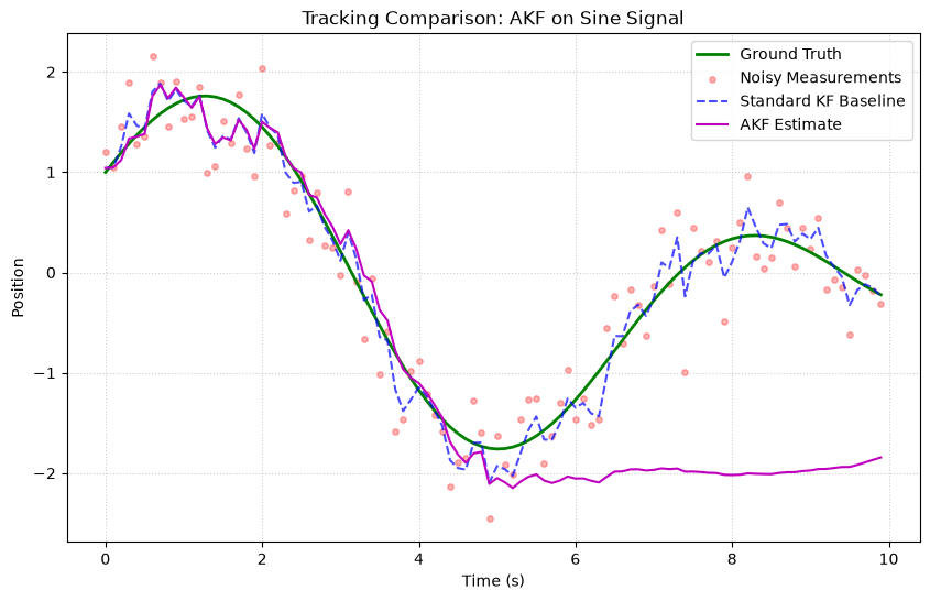
• Analysis: The Adaptive KF (AKF) estimates process noise \(Q\) and measurement noise \(R\) dynamically. On the sine wave, it adjusts covariance scaling to track peaks more responsively compared to the fixed-gain standard KF baseline.

2. Polynomial (Degree 2) Signal

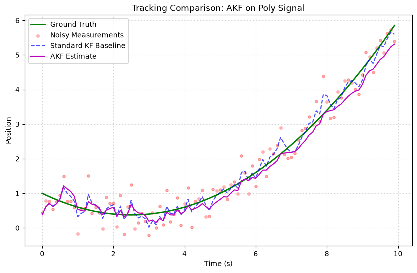
• Analysis: As the target accelerates on the quadratic curve, the AKF detects the increasing residuals, scales up its process noise estimate, and reduces the steady-state lag relative to the baseline KF.

3. Random Walk Signal

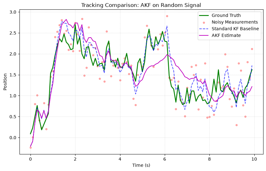
• Analysis: The AKF adapts to local noise shifts stably, maintaining a smooth path without losing track of the true state's random drift.