Alpha-Beta-Gamma Filter (ABG)

The Alpha-Beta-Gamma Filter is a lightweight, fixed-gain filter for tracking position, velocity, and acceleration. It's the simplest filter in kalbee — no matrices, no inversions, just three tuning parameters.

Fundamental Concepts

The Idea

The ABG filter is a simplified form of the Kalman Filter where the gains are fixed rather than computed optimally at each step. It uses three gain parameters:

• α (alpha) — position correction gain
• β (beta) — velocity correction gain
• γ (gamma) — acceleration correction gain

The Algorithm

Predict (kinematic model):

\[ \begin{aligned} \hat{x}_k &= \hat{x}_{k-1} + \hat{v}_{k-1} \cdot dt + \frac{1}{2} \hat{a}_{k-1} \cdot dt^2 \\ \hat{v}_k &= \hat{v}_{k-1} + \hat{a}_{k-1} \cdot dt \\ \hat{a}_k &= \hat{a}_{k-1} \end{aligned} \]

Update (apply corrections using residual \(r = z - \hat{x}\)):

\[ \begin{aligned} x_k &= \hat{x}_k + \alpha \cdot r \\ v_k &= \hat{v}_k + \frac{\beta}{dt} \cdot r \\ a_k &= \hat{a}_k + \frac{\gamma}{2 \cdot dt^2} \cdot r \end{aligned} \]

Gain Tuning Guidelines

Gains	Behavior
High α, β, γ	Fast response, noisy estimates
Low α, β, γ	Smooth estimates, slow response
α = 1, β = 0, γ = 0	Pure position tracking (no prediction)

When to Use

✅ Use ABG when	❌ Don't use when
Low-compute environment	Need optimal estimation (use KF)
Simple kinematic tracking	System is non-linear
Fixed gains are acceptable	Need adaptive noise estimation
Quick prototyping	Multi-dimensional state space

---

How to Use

import numpy as np
from kalbee import AlphaBetaGammaFilter

# State: [position, velocity, acceleration]
state = np.array([[0.0], [0.0], [0.0]])

# Tuning gains
alpha = 0.5    # Position correction
beta = 0.4     # Velocity correction
gamma = 0.1    # Acceleration correction

abg = AlphaBetaGammaFilter(state, alpha, beta, gamma)

# Track a target
dt = 1.0
measurements = [1.0, 2.0, 3.1, 3.9, 5.1, 6.0, 7.2, 7.8, 9.1, 10.0]

for z in measurements:
    abg.predict(dt=dt)
    abg.update(np.array([[z]]), dt=dt)
    pos, vel, acc = abg.x.flatten()
    print(f"Measurement: {z:.1f}  "
          f"Position: {pos:.2f}  Velocity: {vel:.2f}  Accel: {acc:.3f}")

Interface Difference

Unlike other filters, the ABG update() takes an additional dt parameter because the gain corrections depend on the time step.

---

Run an Experiment

The ABG filter is not included in the experiment runner by default (it uses a different state model). You can test it manually:

import numpy as np
from kalbee import AlphaBetaGammaFilter

state = np.array([[0.0], [0.0], [0.0]])
abg = AlphaBetaGammaFilter(state, alpha=0.8, beta=0.5, gamma=0.1)

# Generate sine signal
t = np.arange(0, 10, 0.1)
true_pos = np.sin(t)
noise = np.random.randn(len(t)) * 0.3

errors = []
for i in range(len(t)):
    abg.predict(dt=0.1)
    abg.update(np.array([[true_pos[i] + noise[i]]]), dt=0.1)
    errors.append(abs(abg.x[0, 0] - true_pos[i]))

print(f"Average error: {np.mean(errors):.4f}")

---

Simulation Results

Here is the tracking performance of the Alpha-Beta-Gamma Filter (ABG) compared against the Standard Kalman Filter baseline on three different signal trajectories:

1. Sine/Cosine Signal

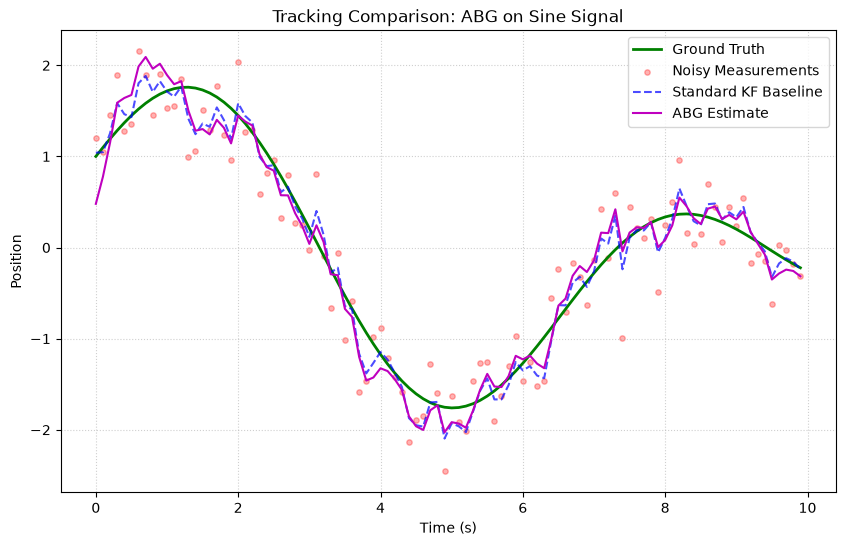
• Analysis: The ABG filter uses fixed gains (\(\alpha=0.4, \beta=0.1, \gamma=0.01\)). It behaves as a simple smooth tracking filter, lagging slightly behind the adaptive Standard KF baseline which changes its Kalman Gain dynamically based on covariance propagation.

2. Polynomial (Degree 2) Signal

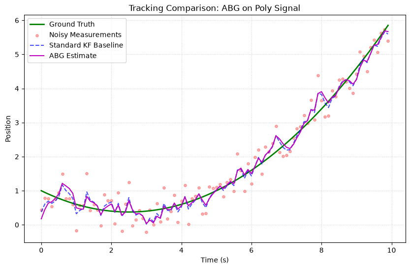
• Analysis: Since the ABG models acceleration with a constant gain factor, it tracks the quadratic curve with less lag than the standard Constant Velocity KF baseline, proving its effectiveness for constant acceleration profiles when properly tuned.

3. Random Walk Signal

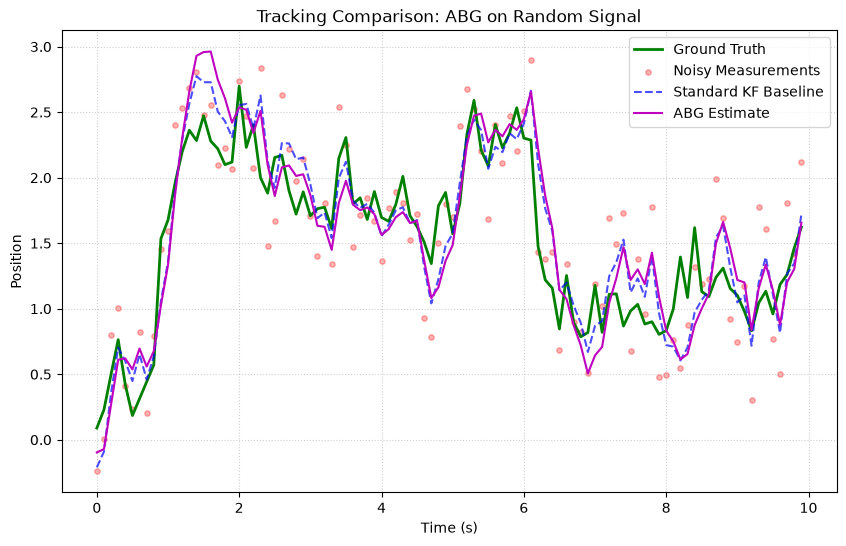
• Analysis: The ABG filter tracks the random walk smoothly, but shows slightly larger deviations than the standard KF since its static gains cannot adapt to changing state uncertainties.