Square-Root Kalman Filter (SRKF)

The Square-Root Kalman Filter (SRKF) is a numerically stable variant of the standard linear Kalman Filter. Instead of propagating the state covariance matrix \(P\) directly, it maintains the Cholesky factor \(S_P\) where \(P = S_P S_P^T\). This formulation prevents the covariance matrix from losing positive-definiteness or symmetry due to floating-point rounding errors.

---

Theory and Formulation

In many tracking scenarios, poorly-conditioned covariance matrices or round-off errors can cause the diagonal elements of \(P\) to become negative, leading to filter crashes. The SRKF mitigates this by maintaining \(S_P\).

1. Predict Step

Given the state transition matrix \(F\) and the process noise Cholesky factor \(S_Q\) (where \(Q = S_Q S_Q^T\)): The predicted covariance Cholesky factor \(S_{P^-}\) is reconstructed using the QR decomposition of a composite matrix:

\[ M^T = \begin{bmatrix} (F S_P)^T \\ S_Q^T \end{bmatrix} \]

A QR decomposition of \(M^T\) yields:

\[ M^T = Q_{qr} R_{qr} \]

The upper triangular matrix \(R_{qr}\) satisfies:

\[ R_{qr}^T R_{qr} = M M^T = F S_P S_P^T F^T + S_Q S_Q^T = P^- \]

Therefore, the predicted Cholesky factor is:

\[ S_{P^-} = R_{qr}^T \]

2. Update Step

Given the measurement matrix \(H\) and the measurement noise Cholesky factor \(S_R\) (where \(R = S_R S_R^T\)): We form the composite update matrix:

\[ A^T = \begin{bmatrix} S_R^T & 0 \\ (H S_{P^-})^T & S_{P^-}^T \end{bmatrix} \]

Computing the QR decomposition of \(A^T\) gives:

\[ A^T = Q_{qr} \begin{bmatrix} X & Y \\ 0 & Z \end{bmatrix} \]

Where: - \(X^T\) is the Cholesky factor of the innovation covariance \(S\). - \(K = (Y^T (X^T)^{-1})^T = Y^T X^{-1}\) is the Kalman gain. - \(S_P = Z^T\) is the updated Cholesky factor of the covariance matrix.

---

Usage Example

import numpy as np
from kalbee import SquareRootKalmanFilter

# Define matrices
state = np.zeros((2, 1))
covariance = np.eye(2) * 10.0
F = np.array([[1.0, 1.0], [0.0, 1.0]])
Q = np.eye(2) * 0.01
H = np.array([[1.0, 0.0]])
R = np.array([[0.1]])

# Initialize and run
srkf = SquareRootKalmanFilter(state, covariance, F, Q, H, R)
srkf.predict()
srkf.update(np.array([[1.5]]))

print("Estimated State:\n", srkf.state)
print("State Covariance:\n", srkf.covariance)

---

Simulation Results

Here is the tracking performance of the Square-Root Kalman Filter (SRKF) compared against the Standard Kalman Filter baseline on three different signal trajectories:

1. Sine/Cosine Signal

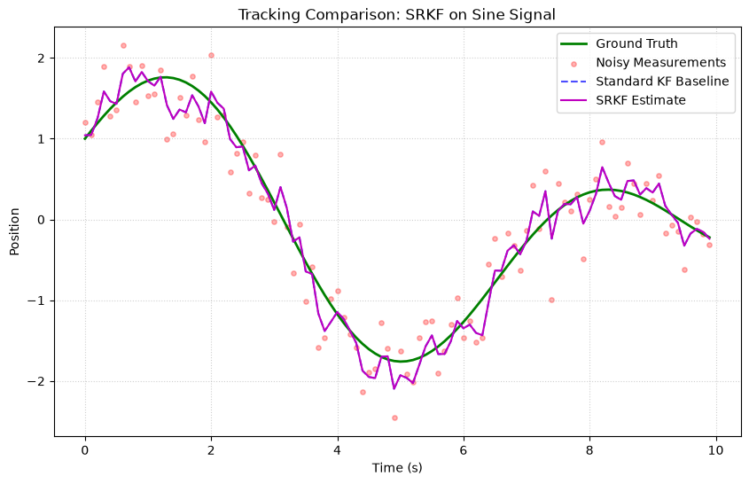
• Analysis: The SRKF maintains the Cholesky factor \(S_P\) instead of the covariance matrix \(P\). In this double-precision simulation, its estimates align exactly with the standard KF baseline.

2. Polynomial (Degree 2) Signal

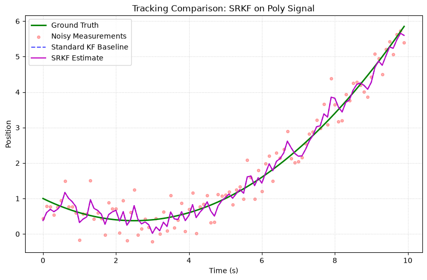
• Analysis: During polynomial tracking, the SRKF mirrors the baseline's steady-state CV model lag, verifying correct mathematical equivalence.

3. Random Walk Signal

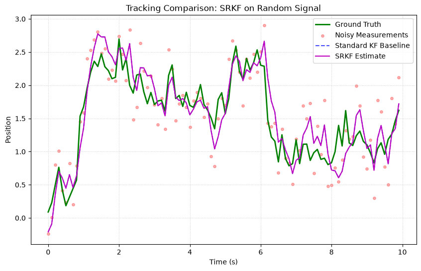
• Analysis: Reconstructs the exact same smoothing path as standard KF while protecting against numerical eigenvalues drift under recursive updates.